(6/20/20) Us modelers are having a field day battling for supremacy. Well I am supreme, but nobody has noticed. So, I made some important upgrades so I am now supremer. Spread the word.
The Problem
Now for some tech talk. There are two camps for COVID-19 modeling trying to be the crystal ball:
- The epidemiologists who have sophisticated kinetic models based on solving several coupled differential equations with many variables, e.g., infectious rate, incubation time, recovery time, population densities, mobility, immunization rates, etc. Their greater value is in taking all the data after the fact and determining all these variables for a particular epidemic and then using them for future (same) epidemics. They say that they can predict based on known previous variables and making certain assumptions, but they don’t predict very far out. These models are sometimes categorized as “dynamic” models, though I never understood what is dynamic about them.
- Then there are the forecasters, like me, who realize that we don’t know all these variables and who only care to forecast ahead using whatever reliable data there is. I chose deaths since they are pretty real and measurable. Others have chosen number of cases, which I have argued is less reliable because it is convoluted with extent of testing and have shown that the reported and real number of cases were off by greater than 10x. They are now generally within a factor of 2-3x, but that is still too large for me. Us forecasters use real-time data and we are categorized as “statistical” models.
The epidemiologists like to criticize these statistical forecasting models because they keep changing their forecasts. Well, that is what forecasts do; would you really not want the weatherman to update things based on new information? Conversely the forecasters cite the litany of unknown variabilities and the inflexibility of epidemiology (let’s shorten to Epi) models as being their shortcomings.
So, at first the two groups defended their corner of the box, but what is reassuring about scientists is that they are by nature introspective and searching for the truth and that the truth doesn’t lie in either of these corners. What is also reassuring is competition, not only to be right, but also not to be wrong. So, what is happening is both groups are seeing the limitations of their models and starting to adopt pieces of the other so that we are now getting hybrid models.
So, this brings us to how I ended up in the middle of the box with a bunch of epi modelers. Despite my being a scientist and needing to understand everything about a process, I am also trying to be pragmatic about solving problems and given that COVID-19 doesn’t give you an eternity to solve a problem, we need to come up with practical tools. This is my business side talking and it seems to mesh well with my science side. So, for this time-critical problem, and not enough time to do a PhD thesis on it (because you know that takes at least 4 weeks), you reach for whatever resources get you the answer. Looking at previous epidemics, and let’s thank China for doing this all for us before they infected the rest of the world, you see that infections and death go up and they go down. Based on the recent China epidemic and also data for the 1918 Spanish Flu these trends look rather Gaussian in shape. So, for forecasting you look for a shape function that is realistic to history and use that to take the emerging data trends and project forward.
The Gaussian model (you know it as the Bell Curve) worked really well on the upside of the epidemic, but with social distancing and then easing, the recovery after the peak of death (and case) rate did not go down symmetrically relative to the rise. So, this was at first easily fixed with an asymmetric Gaussian model that I introduced that gave different rise and fall characteristics. But then this decay shape didn’t match well further into recovery because of persistence in cases and deaths. This is largely due to relaxing of social restrictions.
So how do we deal with this? Epi models don’t usually allow for this changing of their sacred infectious parameter R0 and so they pretty much get it wrong. And a Gaussian model like mine, even adjusted for a different recovery, doesn’t handle the tail very well where deaths are continuing.
Evolution
To better understand the Epi models and where they break down, I programmed the coupled set of differential equations for what is called a SEIR model (Susceptible, Exposed, Infectious, Recovered). You can look up the equations by just Googling SEIR so I won’t show them here. I also added death since that is what we are trying to forecast, but that is easy by just picking a mortality factor for the recovered population. The problem with the standard SEIR model is that the transmission factor R0 is made a constant. SEIR models are intended for epidemics that literally infect everyone so the susceptible population goes to zero and you have herd immunity. There are models that consider not all recovered people getting immunized and they feed back into the susceptible population, but we don’t need to consider this here because we are looking at a range where a minority of the population gets infected. My Gaussian model doesn’t care about the fraction of the susceptible population that gets infected. We just care about deaths and from rates and the total we can derive curves for prevalence (active cases or infectious) and incidence (exposed) as I’ve lectured in earlier posts.
In order to make the SEIR model work better for COVID-19 it needs to have an adjustable R0 representing transmission rate before people realize they need to be careful and here we implement two more R0 values for when social distancing and then easing occur. There then needs to be time for these changes in the equations. Starts to get very complicated. But now the SEIR dynamic model has provisions for statistical forecasting.
The asymmetric Gaussian model I originally postulated had only a single change in transmission rate (our sigma value), which was pegged at the peak of the death rate curve. However, this didn’t account for social easing so I added an additional one. So, the asymmetric Gaussian statistical forecasting model has provisions associated with a SEIR model. However, this is not some amazing unification of diametrically different models because the R0 and our σ values do not have simple relationships. So, for us we consider σ a fitting parameter. The whole point here is to come up with a shape function that fits the previous data and extrapolates well into the future.
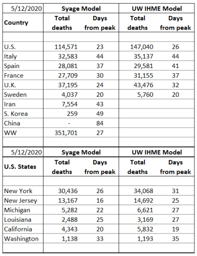
OK, so here are the results. First the table that compares the inputs to the three models described.

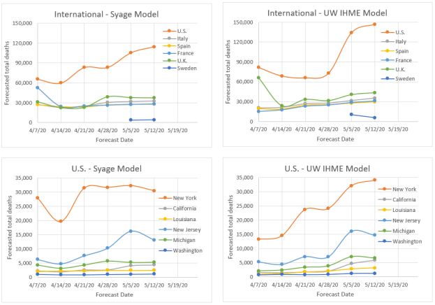
The thing to notice here is we tried to make the inputs as similar as possible between the two models. However, there is not a one-to-one correspondence of variables and as noted above the R0 and σ values, which represent transmission in each model are very different because they plug into very different equations. So, the following plots are for death rate and cumulative deaths by the three models in the above table.

The key observations are:
- The asymmetric Gaussian (red curve) does well fitting to the rise and about halfway down the fall. However, it does not forecast the slowing in the decline of the death rate. This is also seen in the cumulative deaths.
- The SEIR Gaussian and SEIR Statistical models now forecast nearly exactly the same for the parameters in the Table above. The former model may be a little better at the onset of the epidemic as can be seen by a slightly sooner rise by the latter, but this is inconsequential when integrating over the entire death rate curve.
Now we can summarize the forecast of total deaths at various future dates. The intent here was to show that the simpler SEIR Gaussian model and replicate the forecasting of the more complicated SEIR Statistical model and they are very close as you can see, but this was made deliberately. By now having put some SEIR into the Gaussian model we can perhaps anticipate social behavior better. However, we also caution that we are assuming no further social easing, but if social behaviors worsen there could be a much longer death tail and even a resurgence. The UW IHME model, which has consistently under forecasted, a few weeks ago changed their algorithm and now show rampant growth in certain populations (such as CA) that results in much higher forecasted values for all of the U.S. We shall see. As they say “it is difficult to make predictions …. especially about the future.”

The key take home is that the SEIR Gaussian model can offer comparable forecasting power as the SEIR Statistical model. Though it was shown that both approaches offer comparable forecasting capabilities work, our SEIR Gaussian model uses a single function and only needs the variables σ(1), σ(2), σ(3) and τ(2,3). The parameter τ(1,2) can be fixed at zero and the only other variable used, d, is for calculating and forecasting of case prevalence and incidence. The SEIR Statistical Model requires solving five coupled differential equations and requires the variables r, R0(1), R0(2), R0(3), τ(1,2) and τ(2,3).
The scientific version of this description has been posted on MedRxiv (https://www.medrxiv.org/content/10.1101/2020.06.21.20136937v1.article-metrics). The original model can be found on https://www.medrxiv.org/content/10.1101/2020.05.16.20104430v2